LLM Post-Training

Overview

Large Language Models (LLMs) are typically trained in two broad stages: pre-training and post-training.

Pre-training is where the model learns general language understanding from massive amounts of raw, unlabeled text data (Wikipedia, books, GitHub, etc. — often exceeding 2 trillion tokens). The goal is simple: predict the next token given the previous ones. This is an unsupervised learning stage.

$$ \min_{\pi} -\log \pi(\text{I}) - \log \pi(\text{like} \mid \text{I}) - \log \pi(\text{cats} \mid \text{I like}) $$

Here, the model minimizes the negative log-likelihood of each token conditioned on prior tokens — effectively learning grammar, semantics, and world knowledge.

Post-training, on the other hand, refines this general model for specific behaviors, tasks, or human-aligned objectives. It uses curated datasets and sometimes human feedback to make the model more helpful, safe, and controllable.

Post-training Method 1: Supervised Fine-Tuning (SFT)

Supervised Fine-Tuning (SFT) is the first and simplest stage of post-training. The model is trained on a curated set of prompt–response pairs (typically 1K–1B tokens) to follow instructions and generate coherent, context-appropriate answers.

$$ \min_{\pi} -\log \pi(\text{Response} \mid \text{Prompt}) $$

Only the response tokens are used for loss computation — the prompt acts as context.

SFT can be performed via:

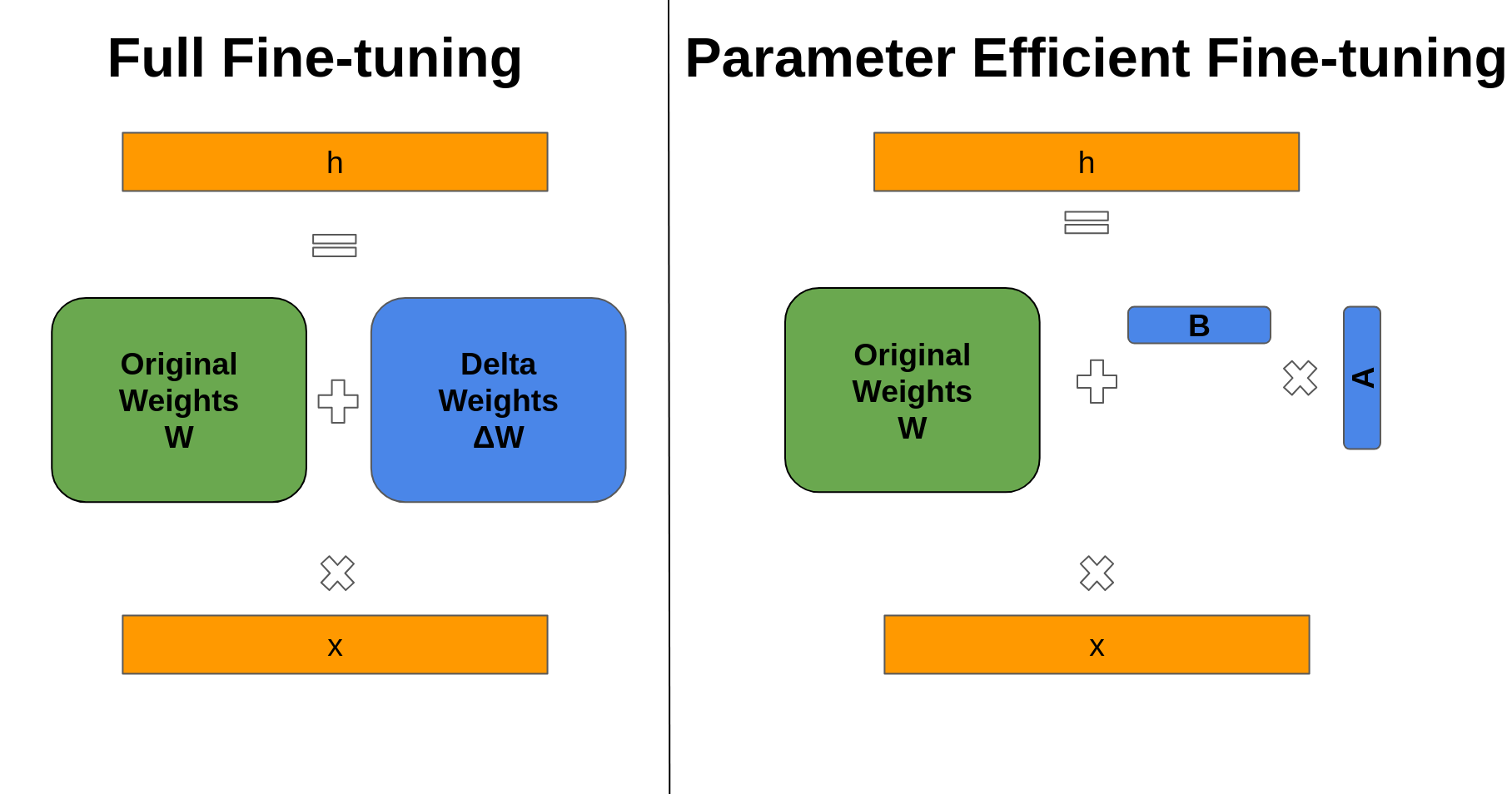
Full fine-tuning: updating all parameters of the model.
Parameter-efficient fine-tuning (PEFT): updating only a small subset (e.g., LoRA, adapters).

Let $h$ be the layer output, $x$ the input, and $W$ the layer’s weight matrix. In full fine-tuning, we update the weights as:

$$ h = (W + \Delta W)x $$

where $\Delta W$ is learned through gradient descent.

In parameter-efficient fine-tuning (e.g., LoRA), we decompose $\Delta W$ into low-rank matrices $A$ and $B$:

$$ h = (W + BA)x, \quad B \in \mathbb{R}^{d \times r}, \, A \in \mathbb{R}^{r \times d}. $$

This reduces the number of trainable parameters from $\mathcal{O}(d^2)$ to $\mathcal{O}(2dr)$, enabling efficient training on smaller hardware.

Full fine-tuning vs. parameter-efficient fine-tuning (LoRA) — Full fine-tuning vs. parameter-efficient fine-tuning (e.g., LoRA).

Post-training Method 2: Direct Preference Optimization (DPO)

Direct Preference Optimization (DPO) simplifies alignment by learning directly from human preference pairs — without explicitly training a reward model or performing reinforcement learning.

Given a prompt $x$, a preferred (positive) response $y_{\text{pos}}$, and a dispreferred (negative) response $y_{\text{neg}}$, DPO optimizes the following contrastive objective:

$$ \mathcal{L}_{\text{DPO}} = -\log \sigma \Big( \beta \big( \log \frac{ \pi_{\theta}(y_{\text{pos}} \mid x) }{ \pi_{\text{ref}}(y_{\text{pos}} \mid x) } - \log \frac{ \pi_{\theta}(y_{\text{neg}} \mid x) }{ \pi_{\text{ref}}(y_{\text{neg}} \mid x) } \big) \Big) $$

Here:

$\sigma$ is the sigmoid function.
$\beta$ controls how strongly the log-ratio difference influences learning.
$\pi_{\theta}$ is the fine-tuned model, and $\pi_{\text{ref}}$ is the frozen reference model (often the SFT checkpoint).

Intuitively, DPO increases the likelihood of preferred responses relative to dispreferred ones while keeping the model close to the reference. It’s simple, stable, and effective for shaping behaviors like helpfulness, harmlessness, or multilingual capability — especially when you have human preference data.

Post-training Method 3: Online Reinforcement Learning (RLHF)

The third and most advanced post-training stage is online reinforcement learning, often referred to as Reinforcement Learning from Human Feedback (RLHF). Here, the model interacts with a reward signal to learn optimal responses.

This process typically involves 1K–10M prompts, depending on the task and resources.

Reward Models and Verifiable Rewards

Given a batch of prompts, the model generates one or more candidate responses. A reward function then scores each response.

Learned reward model: trained on human preference data (humans compare pairs of responses and indicate which is better). The reward model generalizes these preferences to unseen prompts.
Verifiable rewards: automatically computed based on objective criteria — e.g., unit tests for code, accuracy for math, or factual consistency metrics for QA. These remove human subjectivity and are ideal for correctness-based domains.

Policy Optimization Algorithms

Two main policy optimization methods are used in RLHF for LLMs:

PPO (Proximal Policy Optimization)
GRPO (Group Relative Policy Optimization)

PPO (Proximal Policy Optimization)

Given a query $q$, a policy model (LLM) generates a response $o$. Three models interact during PPO:

Reference model: a frozen copy of the base model; used to compute a KL penalty to prevent the fine-tuned model from diverging too far.
Reward model: produces scalar rewards based on human or verifiable feedback.
Value (critic) model: estimates token-level expected rewards to distribute credit across the sequence.

The advantage $A_t$ is computed using Generalized Advantage Estimation (GAE) to quantify how much better each token’s action was compared to expectation.

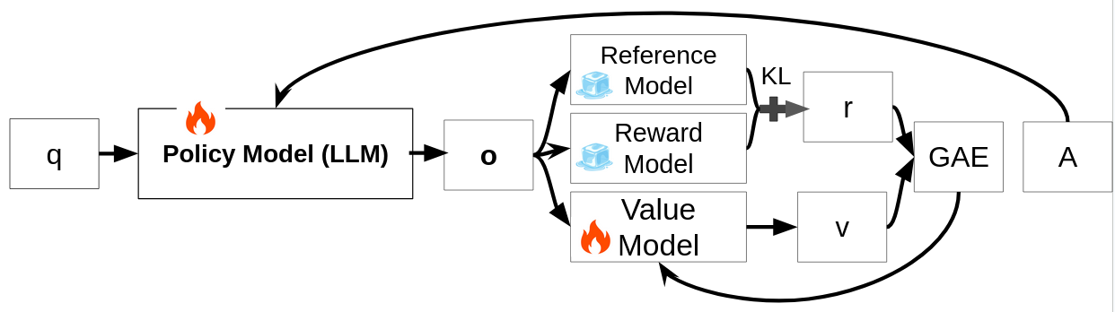
PPO: Reinforcement fine-tuning with reward and KL regularization.

The PPO objective is:

$$ \mathcal{J}_{\text{PPO}}(\theta) = \mathbb{E}_{q \sim P(Q),\, o \sim \pi_{\theta_{\text{old}}}(O \mid q)} \Bigg[ \frac{1}{|o|} \sum_{t=1}^{|o|} \min\!\Bigg( \frac{ \pi_{\theta}(o_t \mid q, o_{\lt t}) }{ \pi_{\theta_{\text{old}}}(o_t \mid q, o_{\lt t}) } A_t, \text{clip}\!\Bigg( \frac{ \pi_{\theta}(o_t \mid q, o_{\lt t}) }{ \pi_{\theta_{\text{old}}}(o_t \mid q, o_{\lt t}) }, 1 - \epsilon, 1 + \epsilon \Bigg) A_t \Bigg) \Bigg] $$

Maximizing this objective encourages responses with higher rewards while maintaining stability through clipping and KL regularization.

GRPO (Group Relative Policy Optimization)

GRPO modifies PPO by changing how advantages are calculated. Instead of using a value model, it generates multiple responses $o_1, \ldots, o_G$ for each query and computes group-level relative rewards. The advantage for each response is derived by comparing its reward to others in the group.

This removes the need for a separate value model, resulting in:

Memory efficiency: no critic model required.
Faster training: fewer model evaluations per step.
Simpler pipeline: advantage estimated via group normalization.

GRPO: Reinforcement fine-tuning with reward.

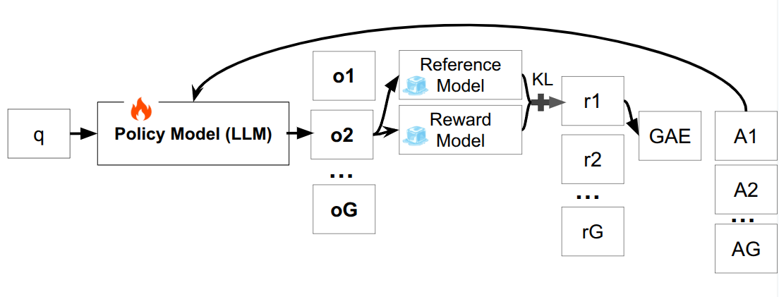
However, GRPO relies on having multiple responses per prompt, making it less suitable when only one response can be sampled.

When to Use PPO vs. GRPO

PPO: Best when fine-grained stability and accurate token-level credit assignment are needed — e.g., safety alignment, fairness tuning, or precise human preference optimization.
GRPO: Best when efficiency is key and multiple responses can be sampled per prompt — e.g., large-scale online RL for conversational LLMs.

Summary

Post-training is where general-purpose LLMs become usable assistants.

SFT teaches them to follow instructions.
DPO aligns them with human preferences efficiently.
RLHF (PPO/GRPO) fine-tunes them to optimize reward functions directly.

Together, these methods bridge the gap between raw pre-trained models and helpful, safe, and aligned AI systems.