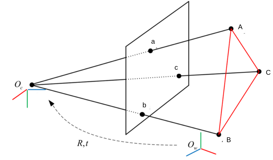
Problem context. On a mobile robot (UAV, rover, AR headset, …) you often know the 3-D world coordinates of a few landmarks \(A,B,C,\dots\) from a prior map. When the on-board monocular camera sees those landmarks again as 2-D image points \(\mathbf a,\mathbf b,\mathbf c,\dots\), the goal is to recover the camera pose \((\mathbf R,\mathbf t)\) that aligns the map with the live view—this is the classic PnP (Perspective-n Point) problem.
In RANSAC-style pipelines you repeatedly sample the smallest number of correspondences needed to determine a candidate pose, test it against all features, and keep the best. Once the intrinsics \(\mathbf K\) are known, you only need 3 points to solve PnP. That minimal subproblem is called P3P, and having a fast, robust solver for it is key to real-time visual SLAM.
We have a camera center \(O\) and three known 3-D landmarks \(A,B,C\). The camera measures unit bearing vectors \(\mathbf a,\mathbf b,\mathbf c\) pointing toward \(A,B,C\). From these we compute the inter-vector angles
\[ \gamma = \angle(\mathbf a,\mathbf b),\quad \alpha = \angle(\mathbf b,\mathbf c),\quad \beta = \angle(\mathbf a,\mathbf c). \]These angles come directly from the image; what remains unknown are the three distances \(OA, OB, OC\).
In triangles \(OAB\), \(OBC\), and \(OAC\), the Law of Cosines gives:
\[ OA^2 + OB^2 - 2\,OA\,OB\cos\gamma = AB^2, \] \[ OB^2 + OC^2 - 2\,OB\,OC\cos\alpha = BC^2, \] \[ OA^2 + OC^2 - 2\,OA\,OC\cos\beta = AC^2. \]Define normalized distances
\[ x = \frac{OA}{OC},\quad y = \frac{OB}{OC}, \]and squared‐length ratios
\[ v = \frac{AB^2}{OC^2},\quad u = \frac{BC^2}{AB^2},\quad w = \frac{AC^2}{AB^2}. \]Since \(u\,v = BC^2/OC^2\) and \(w\,v = AC^2/OC^2\), divide the above three cosine laws by \(OC^2\) to obtain
\[ x^2 + y^2 - 2\,x\,y\cos\gamma = v, \tag{1} \] \[ y^2 + 1 - 2\,y\cos\alpha = u\,v, \tag{2} \] \[ x^2 + 1 - 2\,x\cos\beta = w\,v. \tag{3} \]From \((1)\) we get
\[ v = x^2 + y^2 - 2\,x\,y\cos\gamma. \]Substitute into \((2)\) and \((3)\):
\[ y^2 + 1 - 2y\cos\alpha - u\bigl(x^2 + y^2 - 2xy\cos\gamma\bigr) = 0, \] \[ x^2 + 1 - 2x\cos\beta - w\bigl(x^2 + y^2 - 2xy\cos\gamma\bigr) = 0. \]Collecting terms yields the two‐variable system:
\[ (1-u)\,y^2 + 2u\,xy\cos\gamma -2y\cos\alpha -u\,x^2 +1 = 0, \] \[ (1-w)\,x^2 + 2w\,xy\cos\gamma -2x\cos\beta -w\,y^2 +1 = 0. \]The first equation is quadratic in \(y\):
\[ (1-u)\,y^2 + \bigl(2u\,x\cos\gamma - 2\cos\alpha\bigr)\,y + (1 - u\,x^2) = 0. \]By the quadratic formula:
\[ y = \frac{2\cos\alpha \pm \sqrt{\,4\cos^2\alpha -4(1-u)(1-u x^2)\,}}{2(1-u)} = \cos\alpha \pm \sqrt{\,u\,v - \sin^2\alpha\,}, \]choosing the sign that yields \(y>0\).
An identical step on the second equation gives:
\[ x = \cos\beta \pm \sqrt{\,u\,v - \sin^2\beta\,}, \]again selecting the physically valid root. Finally, recover \(v\) from \((1)\), then \(\;OC=\sqrt{AB^2/v},\quad OA=x\cdot OC,\quad OB=y\cdot OC.\)