
A comprehensive guide to probability theory and statistical estimation for robotics
In this tutorial, I will go over some of the fundamental statistics that every roboticist will encounter at some point in their life. I am assuming the audience will know basic high school statistics and probability theory.
No sensor is perfect! Imagine Rami bot, a rumba-like robot with a sonar distance sensor attached. Using the sensor we wanted to predict where the obstacles are with respect to the world frame (start point of the Rami). Since the sensor is not perfect, it might be noisy and predict the obstacle distance to be 1ft short than what it is.
To help improve Rami's obstacle estimates, being able to quantify the location of the obstacle is important to avoid crashes. For example, it would be helpful to Rami if we can say that the obstacle is ±0.5 ft with a confidence of 90%. This is much more useful for predicting and planning a possible route compared to the deterministic value we get from noisy measurements. This framework can be achieved using probability theory.
Let \(s_i\) denote a possible outcome of an experiment. The collection of \(s_i\) denoted by \(S\) should be such that \(s_i\) are:
Example: Coin flip
Possible samples in the experiment are either heads or tails
\(S =\) { tails, heads}
\(A =\) event heads → {heads}
Notation: In literature, it is conventional to use capital letters to indicate random variables.
Example: Coin flip
\(X =\) {heads, tails}
If it takes a specific value, we indicate by \(P(X=\) heads) i.e., probability of getting heads.
Properties:
For simplicity, instead of using \(P(X=x)\) from here, I will use \(P(x)\)
The probability density function is defined as:
where \(F(x)\) is the probability distribution function.
In the robotics community, the Gaussian/normal density function is widely used.
Parametrized by \(\mu\): mean, \(\sigma^{2}\): variance
Multi-variate case:
Here \(\boldsymbol{x}\) is a vector instead of a scalar
\(\boldsymbol{\Sigma}\) is called the covariance matrix.
Properties:
Don't worry if the above equation looks daunting. You'll see it in various books and will get comfortable with it over time. The key takeaways are the properties of the covariance matrix, and that the two parameters—mean and variance—are all that's needed to define a normal distribution for a state \(x\).
Often random variables carry information about other random variables. For example, LIDAR measurements can carry information about the robot's position.
\(p(x\mid y) = p(X = x\mid Y = y)\) i.e., probability of x given y
If x and y are independent:
Therefore:
This makes sense, right? If \(y\) has no information about \(x\), then querying \(y\) won't contribute anything.
Below are the most used theorems in solving probabilistic proofs and problems in various books:
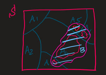
\(B\) is the disjoint union of the intersection \((B \cap A_{i})\) i.e.,
Generally, we can formulate as follows:
Sometimes the above can be written as follows:
The Bayes rule can also be used for more than one random variable:
Property:
Measures squared expected deviation \(\sigma\)
Properties:
If \(\sigma(x,x) = 0\) then the random variable is constant.
If a vector of random variables is transformed by a linear transform \(A\), then the covariance is also transformed as \(\Sigma(Ax) = A \Sigma(x) A^T\)
Measures information content
This can be very useful for estimating the gain of information when our Rami takes a specific action. Usually, we seek to minimize the entropy to increase the gain of information.
The Bayes filter is the foundation for many robotics algorithms including Kalman filters, particle filters, and more. We'll explore these in future tutorials.